
2D Wave equation solver with MPI and HDF5
Overview
This project implements a 2D wave equation solver using the second-order accurate central difference method and MPI-based domain decomposition. The simulation domain in the X-direction is split across distributed-memory ranks, with ghost-cell synchronization at each time step. The output generated is written to an HDF5 file. The entire code is written in Fortran.
The PDE that is beign solved is:
\(u_{tt}(x,y,t) = c^{2}\left(u_{xx}(x,y,t) + u_{yy}(x,y,t)\right) + S(x,y,t)\)
where, \(u(x,y,t)\) is displacement of the wave and \(S(x,y,t)\) is a source function, in this case it’s approximated as a sinusoidal function of \(t\).
The discretized equation is:
\[u^{n+1}_{i,j} = 2u^{n}_{i,j} - u^{n-1}_{i,j} + c^{2}\frac{\Delta t^{2}}{\Delta x^{2}} \left(u^{n}_{i+1,j} + u^{n}_{i-1,j} + u^{n}_{i,j+1} + u^{n}_{i,j-1} - 4u^{n}_{i,j}\right) + \Delta t^{2} S^{n}_{i,j}\]Goals
- Understand and implement MPI parallelization
- Understand and impelemnt HDF5 file format for simulation output
Simulation Setup/Output
Setup
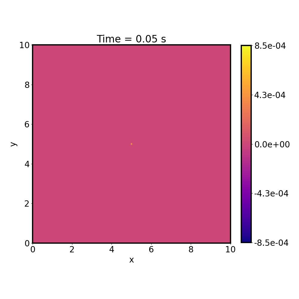
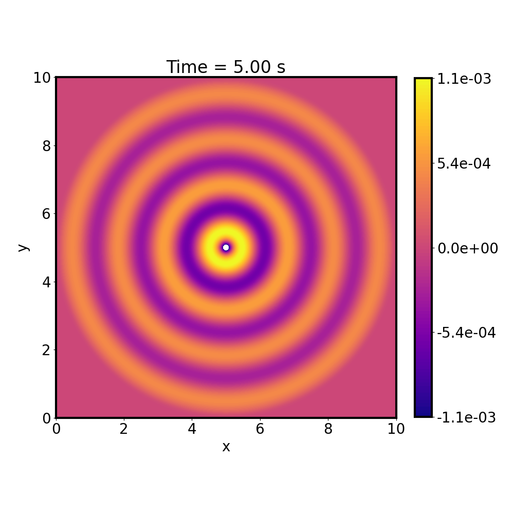
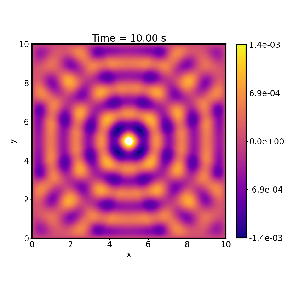
The simulation is setup with reflecting boundary conditions in all the spatial directions. Additionally, a sinusoidal source function is placed at the center of the computational domain, which continuously produces an outward moving wave. As the outward moving wave hits the domain boundary, it gets reflected and interferes with the outgoing wave. This leads to the formation of patterns that we see in the movie.
Output