Multidimensional Ideal MHD solver

Overview

This project initially started as a fun project to build intuition for compressible hydrodynamics and the numerical algorithms behind finite volume methods. As I got more interested in magnetohydrodynamics, I extended the solver from ideal HD (Euler) to ideal MHD by adding magnetic field evolution and the associated Lorentz force terms. To control numerical divergence errors and enforce the solenoidal constraint \(\nabla\cdot\mathbf{B}=0\), I implemented the Generalized Lagrange Multiplier (GLM) divergence cleaning approach. The entire codebase is written in Fortran and is available here.

The code uses MPI for domain decomposition in X and Y directions. Each sub-domain is offloaded to a single MPI core. To futher increase the speed of computation, the computation kernels are offloaded to GPUs using OpenMP offloading. This makes the code GPU architecture independent and provides a speed-up of 10X.

The general MHD Equations in conservaive form are (with permeability \(\mu_{0} = 1\)):

Continuity (mass conservation)

\(\frac{\partial \rho}{\partial t} + \nabla\cdot(\rho \mathbf{v}) = 0\)

Momentum conservation

\(\frac{\partial (\rho \mathbf{v})}{\partial t} + \nabla\cdot\left[\rho\,\mathbf{v}\mathbf{v} + \left(p + \frac{B^{2}}{2}\right)\mathbf{I} - \mathbf{B}\mathbf{B}\right] = \nabla\cdot\mathbf{\Pi} + \rho \mathbf{g}\)

Induction equation (finite resistivity)

\(\frac{\partial \mathbf{B}}{\partial t} = \nabla\times(\mathbf{v}\times\mathbf{B}) - \nabla\times\left(\eta\,\nabla\times\mathbf{B}\right)\)

Divergence free constraint (no magnetic monopoles)

\(\nabla\cdot\mathbf{B} = 0\)

Total energy conservation

The total energy density is defined as \(E = \rho e + \frac{1}{2}\rho v^{2} + \frac{B^{2}}{2}\)

and we evolve \(\frac{\partial E}{\partial t} + \nabla\cdot\left[\left(E + p + \frac{B^{2}}{2}\right)\mathbf{v} - (\mathbf{v}\cdot\mathbf{B})\mathbf{B}\right] = \nabla\cdot(\mathbf{\Pi}\cdot\mathbf{v}) + \nabla\cdot(\kappa \nabla T) + \eta\,|\mathbf{J}|^{2} + \rho \mathbf{g}\cdot\mathbf{v}\)

where the current is \(\mathbf{J} = \nabla\times\mathbf{B}.\)

Closure (ideal gas EOS)

\(p = (\gamma - 1)\rho e.\)

where \(\rho\) is mass density, \(\mathbf{v}\) is velocity, \(p\) is thermal pressure, \(\mathbf{B}\) is magnetic field, \(e\) is specific internal energy, \(\eta\) is resistivity, \(\mathbf{\Pi}\) is viscous stress tensor, \(\kappa\) is thermal conductivity, and \(\mathbf{g}\) is gravitational acceleration.

To recover ideal MHD from the general MHD equations, we take the limit of perfect conductivity and remove all explicit dissipative transport. In practice this means setting the resistivity to zero, \(\eta \to 0\), so magnetic diffusion and Joule heating vanish, and dropping viscosity and heat conduction by setting the viscous stress tensor and conductive flux to zero, \(\mathbf{\Pi}\to 0\) and \(\kappa\to 0\). With these assumptions the induction equation reduces to the flux freezing form \(\partial_t \mathbf{B} = \nabla\times(\mathbf{v}\times\mathbf{B})\), and the momentum and energy equations keep only the conservative ideal MHD fluxes.

Physically, this ideal limit implies that magnetic field lines are advected with the fluid, so the field evolves purely by stretching, compression, and advection rather than resistive diffusion. The Lorentz force remains in the dynamics through magnetic pressure and magnetic tension, and the total energy still includes magnetic energy, \(E=\rho e + \frac{1}{2}\rho v^2 + \frac{B^2}{2}\). Numerically, maintaining \(\nabla\cdot\mathbf{B}=0\) is still essential in the ideal system, since it is a constraint that must hold at all times.

To recover ideal hydrodynamics (Euler) from ideal MHD, we remove magnetic effects by setting the magnetic field to zero, \(\mathbf{B}=0\). Then magnetic pressure and magnetic tension terms vanish from the momentum flux, the induction equation is no longer needed, and the total energy reduces to the purely hydrodynamic form \(E=\rho e + \frac{1}{2}\rho v^2\).

After this reduction the governing equations are the standard Euler equations: conservation of mass, momentum, and total (internal + kinetic) energy with an equation of state such as \(p=(\gamma-1)\rho e\). In other words, the only restoring force in compressible ideal HD is the thermal pressure gradient, and the wave families reduce from the MHD set (fast, slow, Alfvén, and entropy) to the hydrodynamic set (acoustic and entropy).

Any additional physics, such as incorporation of nuclear kinetics (nuclear reactions) and radiation transport can be added as source terms to the above equations.

Simulation Setup/Output

Setup

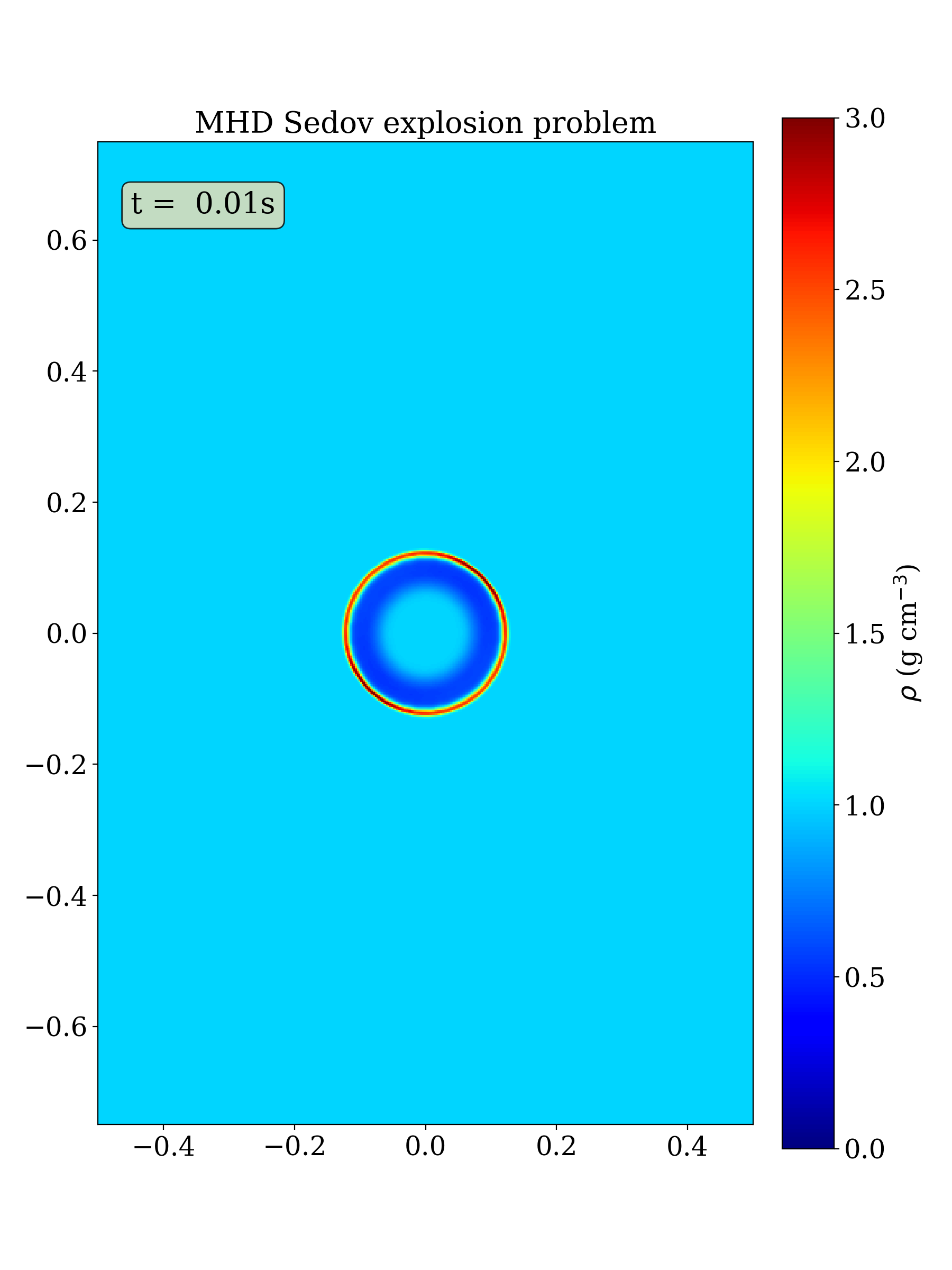
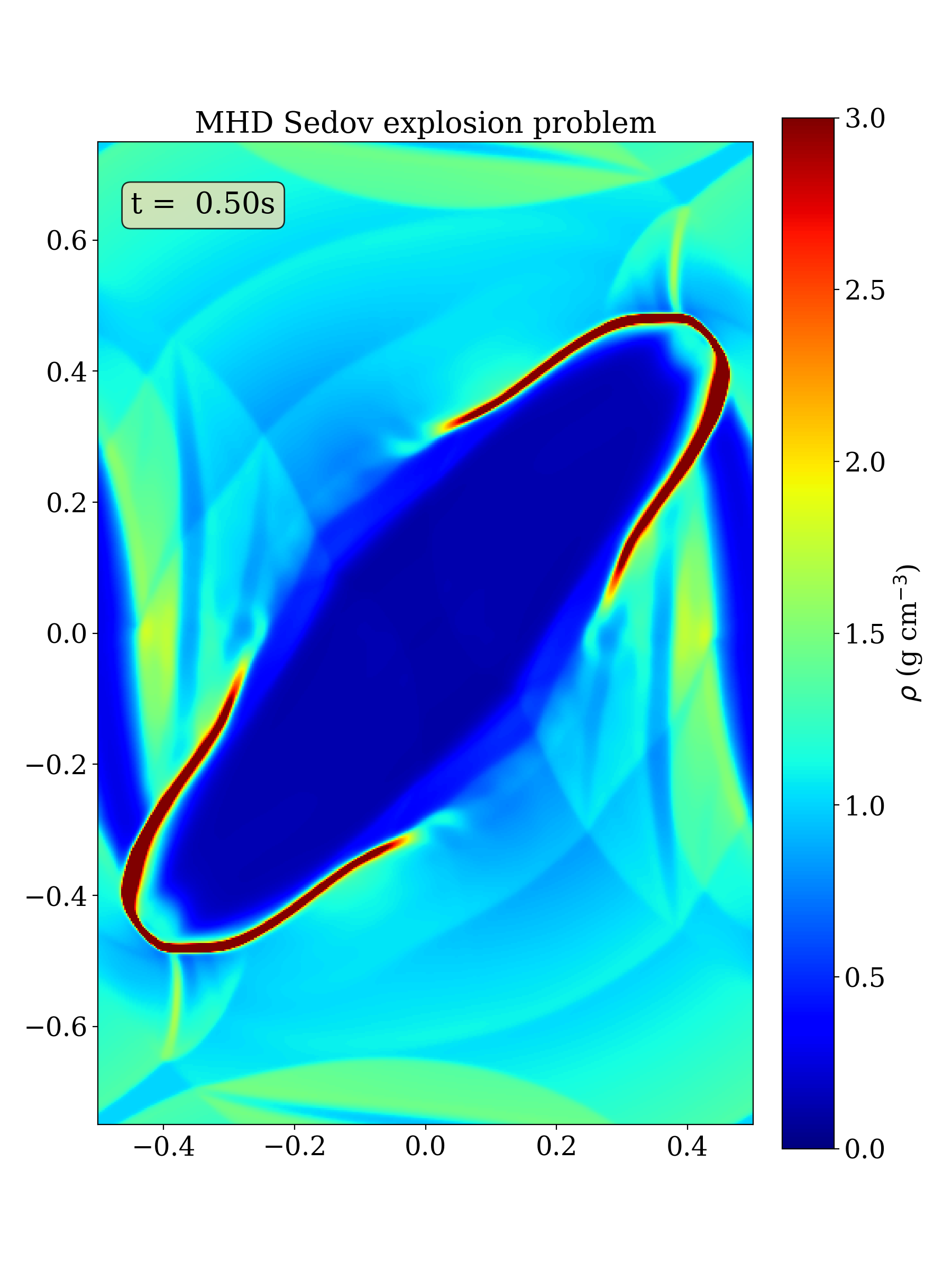
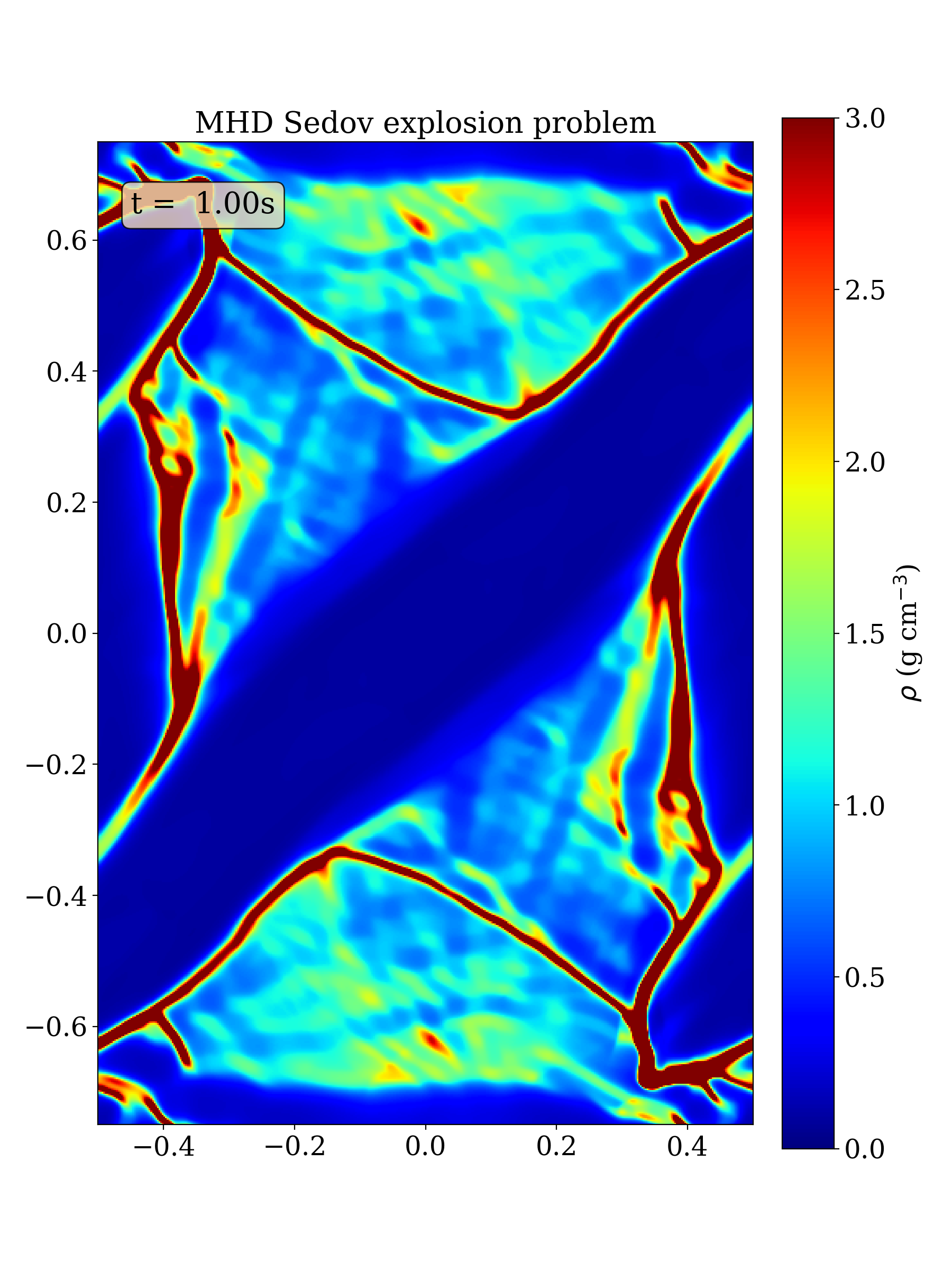
For the Sedov explosion test, I use WENO3 reconstruction with the HLLE approximate Riemann solver in a finite volume framework, with periodic boundary conditions in all spatial directions. Energy is injected at the center of the domain within a small region, launching a strong shock that propagates outward. In the ideal HD case the setup is symmetric, so the shock reaches the domain boundaries at the same time in all directions; with periodic boundaries the outgoing waves re enter the domain and interact with interior structure, leading to Richtmyer-Meshkov instabilities and inner plumes after the shock passes. In the ideal MHD case, in addition to the energy injection, I impose a uniform magnetic field \(\mathbf{B} = \frac{1}{\sqrt{2}}(\hat{i}+\hat{j})\), which breaks spherical symmetry: the shock expands more easily along the field direction and is more strongly compressed across the field, producing a diagonally elongated remnant.

Output

Planned extensions

• Extend the solver to full 3D and also enable a true 1D mode. The core algorithms already support these, but a few code paths and data layouts need to be generalized.

• Write outputs in a standard visualization friendly format that can be opened directly in tools like VisIt.

• Add self gravity. The code currently supports only a constant gravity field, which is useful for tests like Rayleigh-Taylor instability, but I plan to implement a Poisson solver using multigrid for self gravity.

• Extend ideal MHD to resistive MHD by adding finite resistivity in the induction equation and the corresponding Ohmic heating term in the energy equation.

• Add radiation transport, starting with flux limited diffusion and then moving to an M1 closure.

• Add General Relativity (GR) using the Z4c formalism for Einstein equations.